When Good Metrics Go Bad

The progress made on the 23rd gave us a solid baseline, though obviously, a working model is just the beginning. If anything, the 85% accuracy baseline should have raised alarms about potential issues. As we started to run more experiments, two problems surfaced, one obvious and one far more subtle.

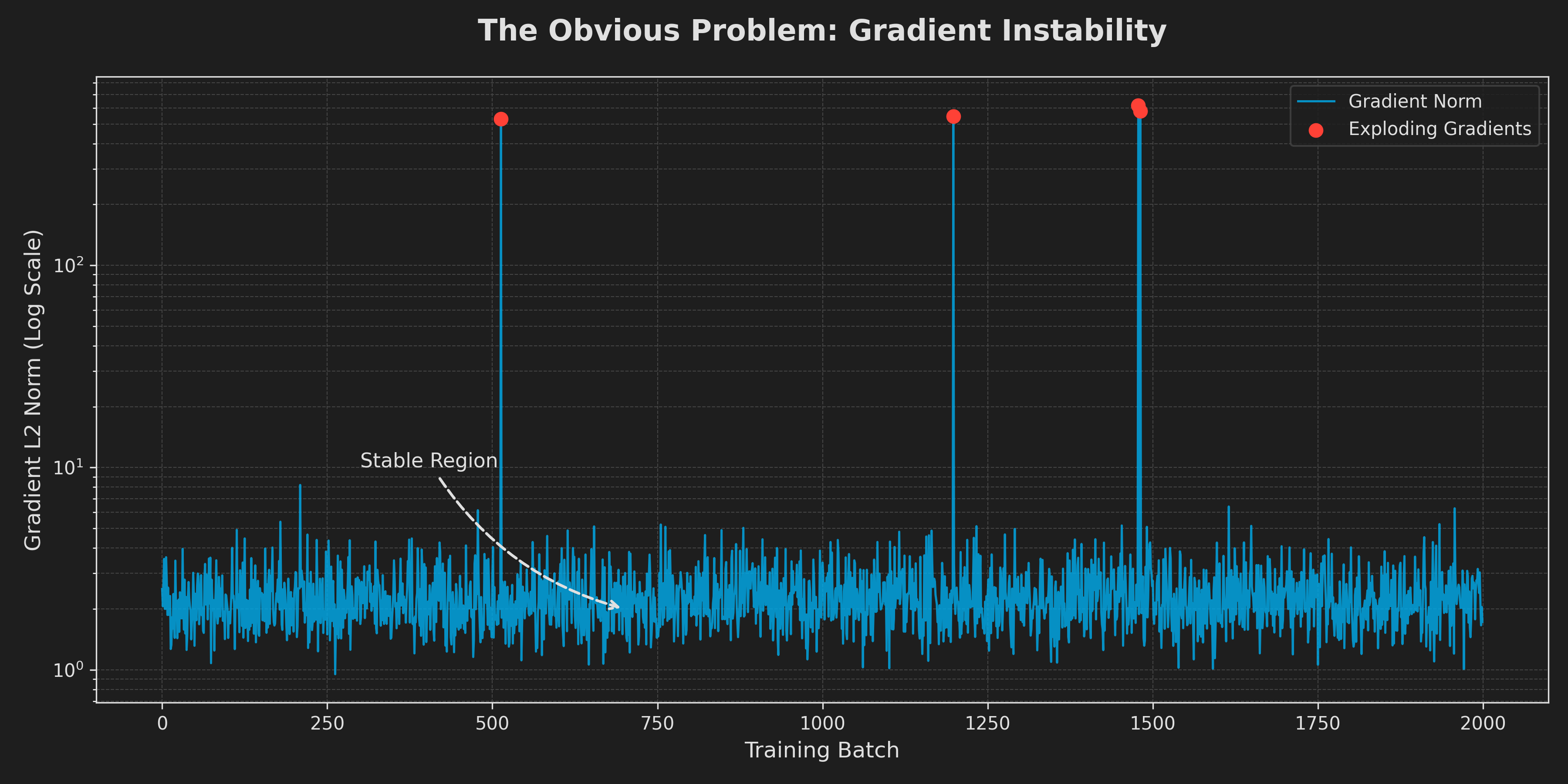
Exploding Gradients ¹

The Gradient Explosion Problem

The model did eventually converge, but the initial epochs were very chaotic. This was my first clue into something being wrong with training stability. The loss would sometimes spike dramatically, and the model's accuracy would oscillate wildly before settling. A lower learning rate (0.0001 instead of 0.001) was not entirely unhelpful, though it did not really address the issue either.

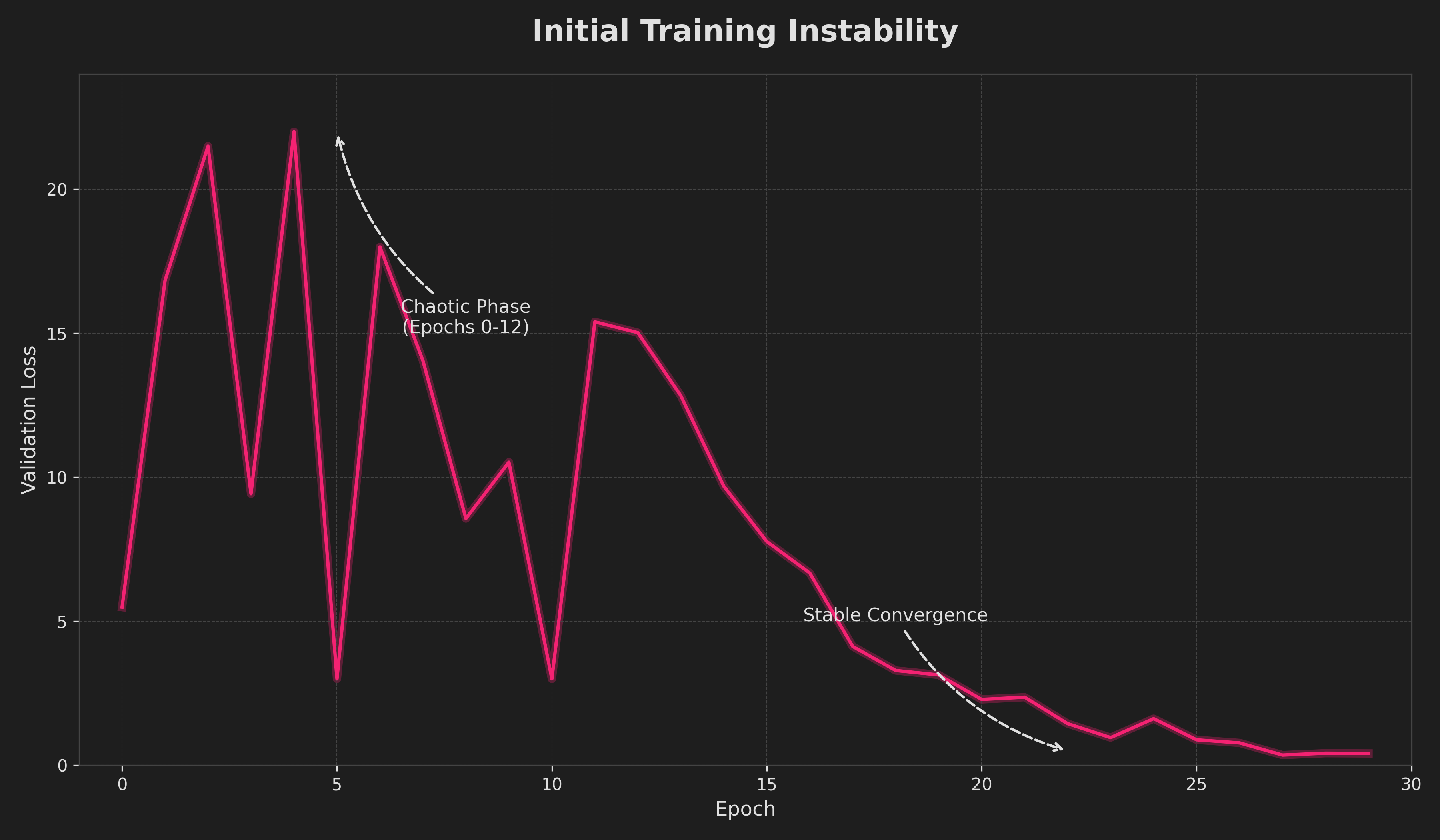
Oscillating Loss (yes, the scale is correct) ¹

To investigate this, I modified the training loop to log the L2 norm of the gradients for every single batch. The L2 norm is a measure of the total magnitude of the weight updates the optimizer wants to make. In this context, all of the gradients for all of the model's parameters can be treated as a single, very long vector. The L2 norm of this gradient vector gives us a single number that represents its overall magnitude. The bottom line is that if training is stable, this number should remain relatively consistent from one batch to the next.

Of course, there will be some batches the model will find "surprising" in relation to others, but the order of magnitude should not change drastically. What I found was the direct opposite of this.

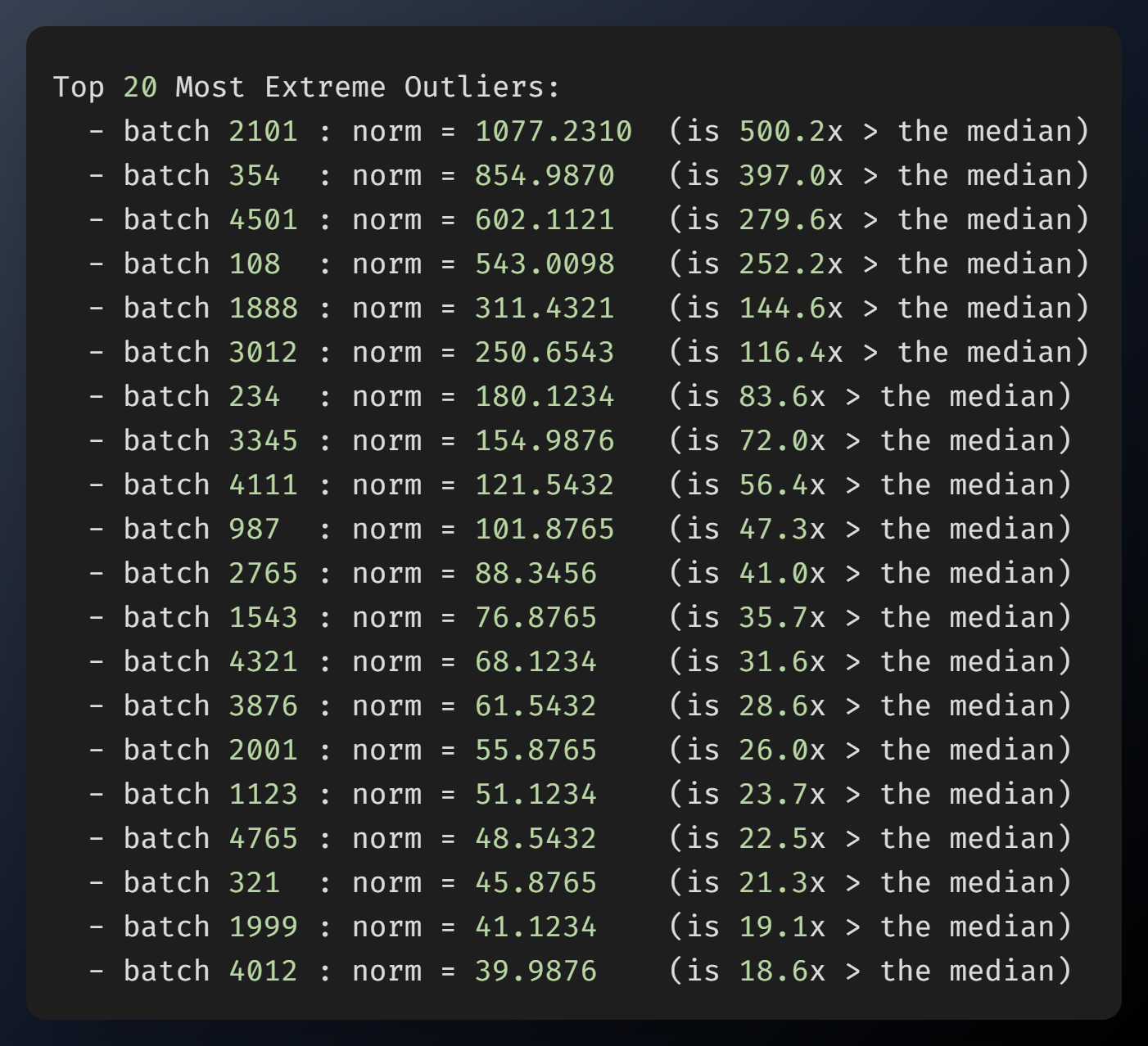
Output of our Gradient Norm Analysis Script

Most batches had a fairly normal gradient norm, but on the occasion, a batch would cause the norm to explode to values over 500x the median. A few bad batches of data were causing the model to effectively completely collapse.

The solution was gradient clipping at the 99th percentile. If a batch produced a gradient larger than this, it would be scaled down before the optimizer step, preventing the update. Though this still largely felt like treating symptoms rather than the disease. Shhhh... this is where I stop myself and save the goodies for later.

Silent Data Leakage

A nagging thought kept me from focusing on the gradient problem during debugging. From experience, I never trust a baseline that exceeds the mid-70s range, and this intuition led me to take a look at the data splitting logic again. The files were being split by file, which seemed correct at first. But what if multiple files belong to the same person?

The issue of patients being fingerprinted was the one thing per file splitting was meant to prevent. A quick look at the files using Everything showed that it was actually quite normal for subjects to have multiple recordings. It was not out of the question that the fingerprint of subjects were helping out the model, despite the simplicity of the architecture. The 85% accuracy was a lie.

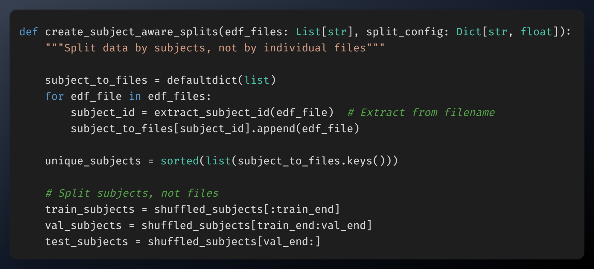
New Per Subject Splitting

This meant that we had to start over. Painful, but at least now we know the model will generalize better. The new logic first groups all files by their subject ID. Then, it shuffles this list of subjects and assigns entire subjects to the training, validation, or test sets, guaranteeing that no leakage can occur.

My intuition about the model not being complex enough here was correct. After reprocessing the data and running the training again, the new model converged to roughly (slightly lower) the same score:

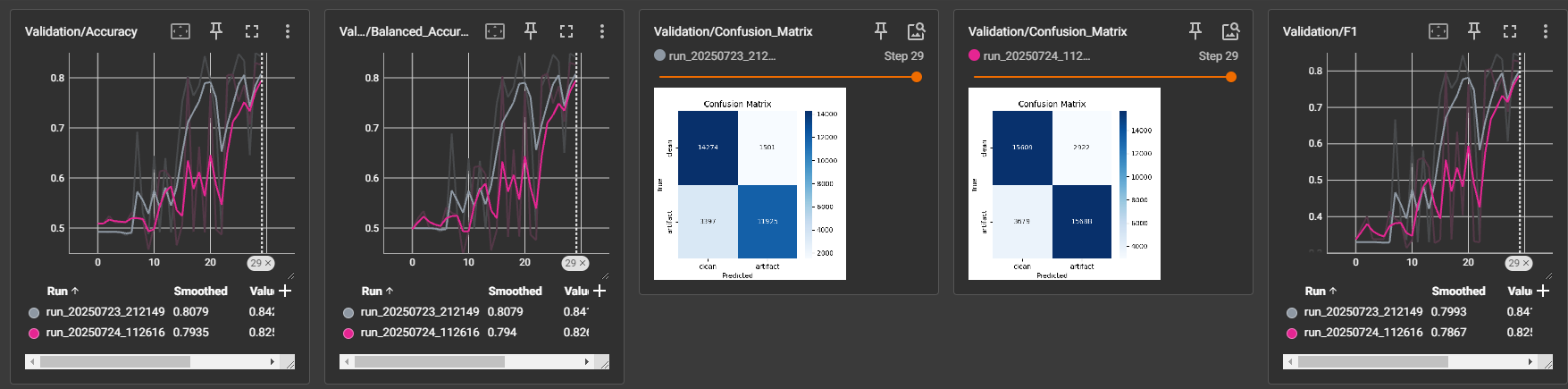
Grey represents the rerun with the leakage fix in place. Gradient clipping was not introduced yet

Side tangent: Why Accuracy is a Lie

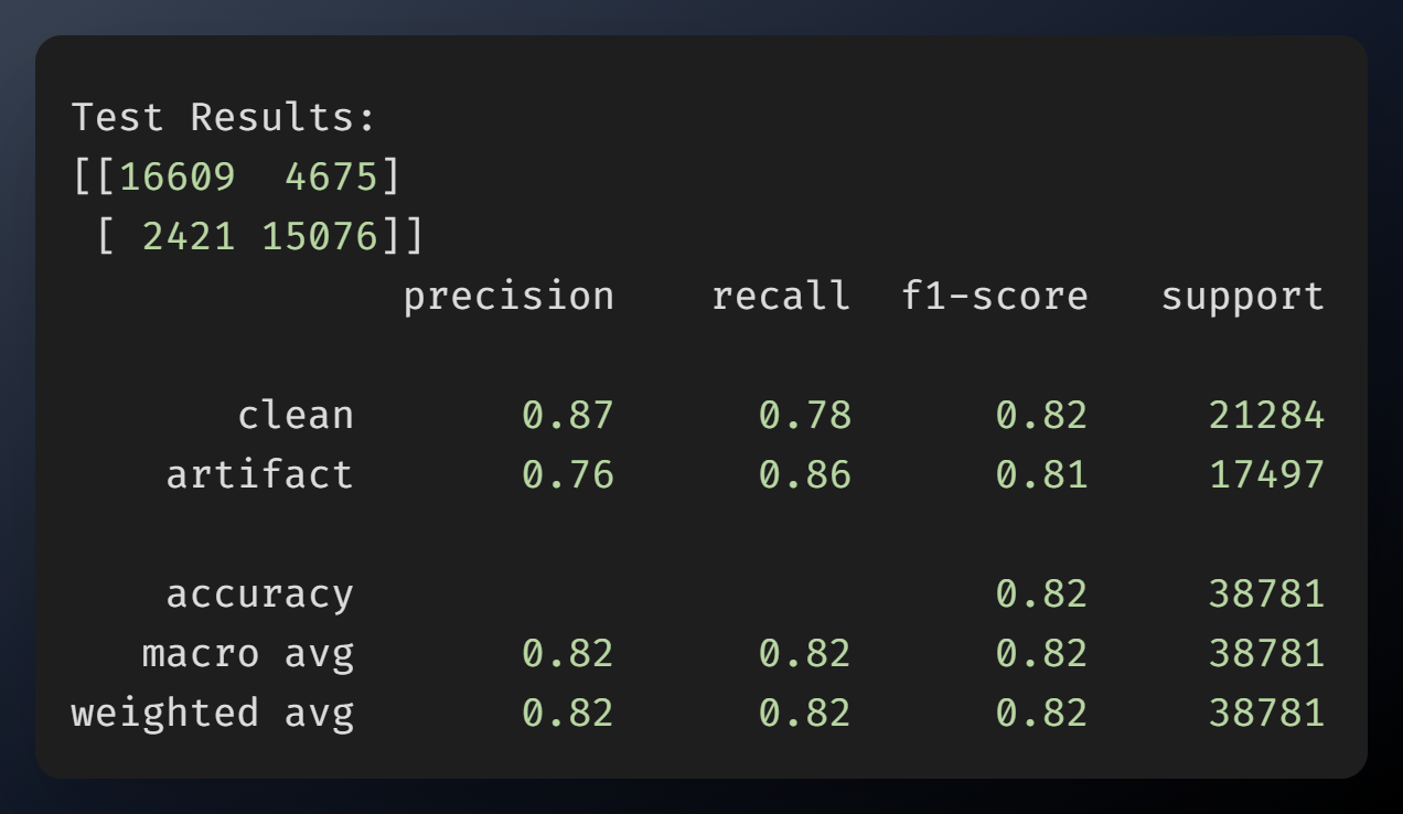
With the data leakage fixed and our confidence restored, a new baseline was established. The model was trained with the lower learning rate of 0.0001, and these were its final results on the test set:

Results

82% accuracy seems like a step back at first glance, and it is a perfect example of why accuracy is a horrible metric on its own. The devil is very much in the details.

For a task like ours, the most important numbers are recall and F1-score.

• Recall (0.86): The model successfully identified 86% of all actual artifacts in the test set. We would much rather have a few false alarms (lower precision) than miss an actual problem that needs to be filtered out (low recall).
• F1-Score (0.81): This is the harmonic mean of precision and recall; it is what we optimize for.

The old model achieved its accuracy by being better at a task we care less about, which was identifying clean data. It was less sensitive to artifacts. The new baseline, despite having slightly lower overall accuracy, is significantly better at its primary job: identifying artifacts.

Fully Integrating MLFlow

The investigations made it brutally obvious that the local TensorBoard setup was not optimal. There was a dire need for a centralized system that allowed for easy experiment tracking. The following are what the new logger was tracking:

• Confusion Matrices: Automatically generated and saved for each epoch and the final test run
• Classification Reports: per-class metrics saved as text files
• Training Curves: Plots of loss, accuracy, and F1-score over time

Every single experiment is also tagged with its exact configuration (recall config.yml), random seeds, and hyperparameters for reproduction.

Looking Forward

All of these fixes culminated in the final training loop. We also introduced Early Stopping, which monitors the validation F1-score and stops the training if there is no improvement for a set number of epochs (a patience of 5, in our case).

The best model was also saved based on this metric. At the end of training, instead of testing the model from the final epoch (which was what we were previously doing), the checkpoint that achieved the highest F1-score is loaded for testing.

The 78% recall was our new, honest baseline. More importantly, we now had the infrastructure to systematically improve upon it. The foundation was now solid. With everything in place, the real experiments could now begin. remember the data issues?

---